CSC 101 CompLit, Fall
1996
Merrie Bergmann
Ileana Streinu
Dominique Thiébaut
Lab 2
Thursday, September 12,1996
Diskette preparation
Word Processing
Spreadsheet
Drop Box
0. Diskette preparation.
Insert your diskette. If this is a new
disk, it will ask if you want to initialize it: say yes. If it
gives you an option, choose two-sided. Name the diskette something
like "Jean Smith: CSC101," so that if you lose it, it
can be identified. Erase the diskette and rename it by editing
the name under the diskette icon (click on it, wait until it changes
color, then edit it).
This process should be repeated for
each lab partner, although you only need one diskette for this
lab.
1. Word Processing
0. Logon to the Seelye server, as you
did last week. (Look up in Lab1 if you forget how.)
1. Find the file "L2.Word"
in SeelyeCourseware/Literacy. Copy this to your diskette by dragging
its icon on top of your diskette icon (the point of the cursor
arrow is the active part).
2. Double-click on the
" "
icon (Microsoft Word 5.1), which is located at top-level folder in
Seely.Mac (Do NOT use the newer version Microsoft Word 6.0.1. for this assignement, although you can experiment with it later on your own). You should see a document named "Untitled 1".
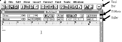
The line of icons just below the menu bar is called the "Tool
bar." The line below the document name is called the "ribbon,"
and the graduated line below that is called the "Ruler."
"
icon (Microsoft Word 5.1), which is located at top-level folder in
Seely.Mac (Do NOT use the newer version Microsoft Word 6.0.1. for this assignement, although you can experiment with it later on your own). You should see a document named "Untitled 1".
The line of icons just below the menu bar is called the "Tool
bar." The line below the document name is called the "ribbon,"
and the graduated line below that is called the "Ruler."
Turn on Balloon Help and figure out
what the symbols on the Tool Bar mean. Then you can either leave
Balloon Help on or turn it off, whichever you prefer.
3. Close the Untitled document; you
won't need it (you learned how to close a document in the Mac
Tour last week).
4. Open the file L2.Word via File/Open.
Now you should have a copy of this document on your screen. It
is the beginning of the novel Ulysses by James Joyce, with
some "paragraph" numbers added for reference.
5. Your task in this part of the lab
will be to modify this file in various ways specified below. Tick
them off as you progress so you don't accidentally miss one!
(1) Change the view to PageLayout. Choose
the option Show¶ (when you select this, it changes to Hide¶,
indicating the next selection will hide the special symbols).
This is perhaps the most convenient way to view a document, as
it shows various otherwise hidden information.
(2) The entire text is in the New York
font, point size 10. Figure out how to select the entire document
(use Balloon Help, hunt around the menus, try things out, recall
what you learned in the Mac Tour). The background is colored when
you have selected it. After selecting, change the font to Helvetica
and the point size to 12. Click anywhere to deselect the text.
(3) Prior to the first line, insert
Ulysses
James Joyce
with the title in bold, the author in italics, both point size 14, centered; include a blank line following the author. You can first
type these three lines, and then change font, size,
and centering (centering tools are on the ruler-- again use Balloon
Help if necessary).
(4) Change all of paragraph
1 to the New York font, and all of paragraph 2 to the Times font.
Select each first, and then change the font.
(5) Change all of paragraph
3 to use "fill" mode (on the ruler), rather than the
"ragged right margin" it was initially.
(6) Change all of paragraph
4 to Outline (you may need to hunt around for this).
(7) Double-space paragraph
5 (that's the wider, right option on the ruler).
(8) Delete paragraph 7
entirely.
(9) Copy paragraph 8 and paste it between paragraphs 2 and
3. Make sure there is no extra line inadvertently inserted.
(10) Place the cursor prior
to the first word, and run the Spelling checker (use Balloon Help
to find it). "Correct" every instance of a word that
Joyce uses as one, but it usually written as two (such as "stairhead").
Perform this correction whether or not the corrector suggests
a separation. Do not correct anything else (Latin, proper names,
etc.).
(11) Grammar check paragraphs
9 and 10. Permit it to change any instances for which it offers
to do so (but enabling the Change button).
(12) Insert a section
break between the centered author name and the first line of the
novel. Now select from paragraph 1 through to the end, but not
including the centered title and author. Finally, change the selected
part to be double-column (icon on the ribbon).
Flip back and forth between
viewing the document under PageLayout and Normal, and Show
and Hide¶ so you see the difference. Leave it in PageLayout
with ¶'s shown.
(13) Insert into the header
"Ulysses" in Greek (point size 14, not bold) using the
Symbol font, like this:

(14) Select File/PrintPreview.
This should show your document to be two pages, the second of
which only the first column contains text. At this point you could
print it out, but I do not care to have a printout, so let's save
some trees.
(15) Finally, please add
your full names to the bottom of the file. You are now finished
editing the document.
6. Select the File/Save as..."
command. Check the dialog box to make sure it is about to save
to your diskette. Use "L2.Word.Name1.Name2" as the name
of your document (where Name1 and Name2 are your last names only,
beginning with uppercase; please have Name1 the alphabetically
first; if yous last name is not unique, please add an initial after your lastname), and click on the "Save" button. Now the file
is saved to your diskette. (You cannot save files directly to
the server [which is why the folders have the slashed-pencil icon],
so if you want to preserve a file, you have to store it either
on the local Mac or on a diskette. The
Mac harddrives are locked, leaving the diskette as your only option.)
7. Quit Word. Check the Applications
icon to make sure you are only running the Finder now.
2. Spreadsheet
In this part of the lab
you will make some spreadsheet calculations and make two charts.
Just in case I don't get to explain this in class beforehand,
I start below with some general instructions on how to use Excel,
followed by specific instructions for this lab. You can skip the
general if you feel ready to tackle the specific.
General
Numbers and text are entered into a
spreadsheet cell by selecting it (by clicking) and typing. Entering
formulas is more difficult. To enter a formula for one cell, first
select it, and second, type an = sign. This tells Excel that you
are not entering data or text, but rather wish to enter a formula.
It jumps the cursor up into the "formula bar."
Now you type an expression representing
the formula, for example, A2+B2, meaning the sum of the number
in column A, row 2, and the number
in column B, row 2. You may edit the formula just as if you were
in Word. When you are satisfied with it, click the check box;
the X box is for canceling the formula enter.
Because it is tedious to type the formulas,
at the point where you would like to enter something like A2,
you can just click on the A2 cell instead, and Excel will type
A2 for you.
Formulas may be copied and pasted elsewhere,
and you will see that Excel is intelligent enough to paste A3+B3
into row 3, rather than A2+B2, if that is what you copied. Also
under the "Edit" menu you will find "Fill down"
and "Fill right", which copy one formula down an entire
column or right an entire row of selected cells, again intelligently.
I encourage you to explore ways to avoid tedious typing, but if
you can't figure it out, then it is OK to type each formula individually.
Specific
1. Find the file "L2.Excel"
in SeelyeCourseware/Literacy. Copy this to your diskette just
as you copied L2.Word above.
2. Launch Excel (just like you did Word),
close the initial Untitled document, and use File/Open to open
L2.Excel on your diskette. You should see three columns of data.
The first is academic year, and the second two are the Fall and
Spring enrollments in Computer Science classes.
3. Add a new column, labeled "Total,"
which contains the total Fall+Spring enrollment. For this you
need to enter a formula into cell D2 and fill it down the column
(see general instructions above if you don't know how to do this).
4. Add two additional columns, labeled
"% Fall" and "% Spring," which show the percent
of enrollments which were in the Fall and Spring respectively.
The relevant formula here is 100*[Fall]/[Total], where I have
left in brackets what you need to specify as cells. E.g. if column
B is labeled "Fall" and column D is labeled "Total",
you should enter 100*B2/D2. Again fill the formulae down.
5. Change these two percentage columns
to have only one decimal place, by first selecting them, and then
using Format/Number... and specifying a Code 0.0 (which is a template
indicating one decimal place).
6. Select all your data and headers
and right-justify. So all the column headings should line
up with the data under it.
7. Now select the column headings and
make them all bold.
8. Select the Years (all but the heading
"Years") in the first column, and using Format/Patterns...
select a light stippling pattern as background for this column.
9. Select all the other data (not the
first row, not the first column, but everything else), and place
a box around it with Format/Border...
10. Now we are going to make a chart.
Select the first three columns of data (Years, Fall, Spring),
excluding the column headers. Now select the "Chart Wizard"
tool on the Toolbar. This changes your pointer to a crosshair.
It is now waiting for you to drag out a box for the chart. Choose
any size you want, and place it anywhere you want.
11. You now will be presented with a
variety of options in several dialog boxes. Make some choices.
You'll get to do it again, so don't worry. When you get a chance
to add a title, entitle the chart "CS Enrollments" and
label the X-axis "Academic Year." When you are through
all your choices, you should have a chart. It is selected, as
indicated by the "handles" (the little square boxes).
12. Delete your chart with Edit/Cut.
Start over and make a nice chart that you feel displays the data
most lucidly or perspicuously. You can move the chart with click
and drag; you can resize it by dragging the handles.
13. Double click on your chart. This
will take you into chart-editing mode, indicated by the chart
appearing as if it is its own window. Now you can click on a colored
region, and change its color or pattern. Explore around here and
make at least some changes to the defaults originally supplied
by the Chart Wizard tool. When you are satisfied, close by clicking
in the upperleft corner.
14. Now I'd like you to make one more
chart. This one will be based on three columns of data, Year,
% Fall, and % Spring. First copy these three columns into a fresh
area of your spreadsheet (scroll down below the chart you already
made). You can copy each column separately. The point of doing
this is to get the three of them adjacent. When you paste the
% columns, choose PasteSpecial and only paste the values (not
the formulas- they won't work when moved).
15. Now select the three columns of
data, and make a nice chart based on them.
16. Please add your full names someplace
near the top of the spreadsheet.
17. Select the File/Save
as..." command. Use "L2.Excel.Name1.Name2" as the
name of your document (where Name1 and Name2, same as before, are your last names
only, beginning with uppercase), and click on the "Save"
button. Now the file is saved to your diskette.
18. Quit Excel. Check
the Applications icon to make sure you are only running the Finder
now.
3. Drop Box
The two files you created
in this lab are due next Thursday. When you are finished with
them, and you have them named correctly (L2.Word.Name1.Name2 and
L2.Excel.Name1.Name2), then drag them to the DropBox in the Literacy
folder. If you get the familiar "copying..." feedback,
it worked. You can look in the DropBox to see if it was deposited,
but there can be so many files in there it is not always easy
to see yours.